another experiment

(This post is an experiment in two senses. First, to test embedding graphs from the Desmos calculator into the post. Second, to show the results of a mathematical experiment carried out on Desmos and Twitter last night.)

In Spivak’s classic textbook Calculus, one exercise asks the reader to show that each of the following (complex) power series has radius of convergence 1: \[ \sum_{n=1}^{\infty} \frac{z^n}{n^2}, \hspace{0.5in} \sum_{n=1}^{\infty} \frac{z^n}{n}, \hspace{0.5in} \sum_{n=1}^{\infty} z^n. \] (I’ll leave that task to you. Hint: ratio test.) Another exercise then says, “Prove that the first series converges everywhere on the unit circle; that the third series converges nowhere on the unit circle; and that the second series converges for at least one point on the unit circle and diverges for at least one point on the unit circle.” Points where a series converges always raise a new problem: can we tell what value it converges to? Generally, that problem is hard. But at a point where a series is known to diverge, the story’s over, right? Well, no. There are many ways for a series to diverge.

I want to focus here on the behavior of $\sum z^n$ when $|z| = 1$. The series diverges, of course, because the size of every term is 1. But what do the partial sums look like? What do their real and imaginary parts look like? My thoughts on this began last night when I plotted the graph of $\sum_{n=1}^{50} \sin nx$:

(Click on the graph to go to an interactive version.) To my surprise, there appeared to be well-defined curves bounding the top and bottom of this graph. To be more precise, the points corresponding to critical values (or local extreme values) of the function lie on a pair of analytic curves. After some playing around, I found these curves to be the graphs of ${-\frac{1}{2}} \tan \frac{x}{4}$ and $\frac{1}{2} \cot \frac{x}{4}$ (shown in blue and green, respectively, below).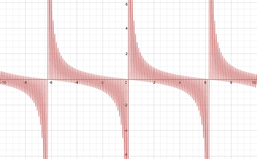

I sent out a tweet about my discovery: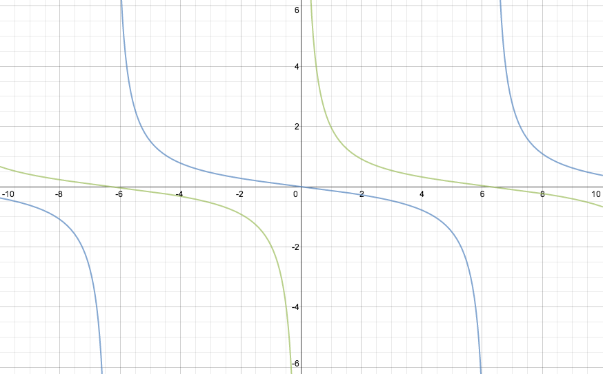

This certainly *looks* like it fits, but I have no idea why. desmos.com/calculator/e67… @desmos #math #mathchat

— Joshua Bowman (@Thalesdisciple) June 11, 2013

I went investigating and found some hints that this behavior might be related to the Fourier series of the cotangent. Meanwhile, my tweet generated some interest, including this response:

@thalesdisciple @desmos Looks like using formula for a partial geometric sum on e^(inx) should explain it?Thanks for posting.Very cool.

— Paul Johnson (@ptwiddle) June 11, 2013

Also, later in the evening, Desmos took my initial graph and augmented it:

@ptwiddle @thalesdisciple What a fun exploration! I added a few things to your original graph. desmos.com/calculator/wz2… #SinesOfMadness

— Desmos.com (@Desmos) June 12, 2013

Paul’s on the right track, which brings us back to the Spivak exercise I mentioned earlier.

To get a point of the unit circle, write $z = \mathrm{e}^{ix}$, with $x \in \mathbb{R}$. Then the summation formula for partial geometric series yields \[ 1 + \mathrm{e}^{ix} + \cdots + \mathrm{e}^{imx} = \frac{1 - \mathrm{e}^{i(m+1)x}}{1 - \mathrm{e}^{ix}}. \] We can take imaginary parts of both sides and use some trig identities to get \[ \sin x + \cdots + \sin mx = \frac{\cos \frac{x}{2} - \cos \big(m+\frac{1}{2}\big)x}{2 \sin \frac{x}{2}}. \] (Note that Desmos included this latter formula in their augmented form of the graph. See also this nice derivation.) On the other hand, the tangent half-angle formulas give us \[ -\tan \frac{x}{4} = \frac{\cos \frac{x}{2} - 1}{\sin \frac{x}{2}} \qquad\text{and}\qquad \cot \frac{x}{4} = \frac{\cos \frac{x}{2} + 1}{\sin \frac{x}{2}}. \] When $\sin\frac{x}{2}$ is positive (for example, when $0 < x < 2\pi$), we have \[ -\frac{1}{2} \tan \frac{x}{4} \le \sin x + \cdots + \sin mx \le \frac{1}{2} \cot \frac{x}{4}, \] with equality on the left whenever $\cos\big(m+\frac{1}{2}\big)x = 1$ and equality on the right whenever $\cos\big(m+\frac{1}{2}\big)x = -1$. The direction of the inequalities is reversed when $\sin\frac{x}{2} < 0$, but the rest of the analysis remains the same. This is the desired result.

Thus the imaginary parts of the partial sums of $\sum \mathrm{e}^{inx}$ are always contained between $-\frac{1}{2}\tan\frac{x}{4}$ and $\frac{1}{2}\cot\frac{x}{4}$. To complete the picture, let's look at the real parts. Here is the graph of $\sum_{n=0}^{50} \cos nx$:

Using similar arguments as before, we can show that the value of $\sum_{n=0}^m \cos nx$ always lies between $\frac{1}{2}-\frac{1}{2}\csc\frac{x}{2}$ and $\frac{1}{2}+\frac{1}{2}\csc\frac{x}{2}$.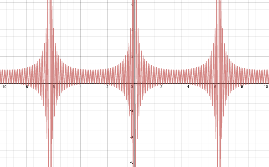

Therefore, even though the series $\sum z^n$ diverges whenever $|z| = 1$, the real and imaginary parts of its partial sums remain tightly constrained by values that depend analytically on the argument of $z$ (unless $z = 1$, i.e., its argument is a multiple of $2\pi$, in which case the series is just $1 + 1 + 1 + \cdots$).

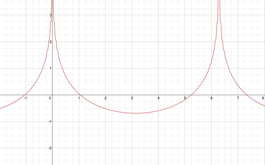
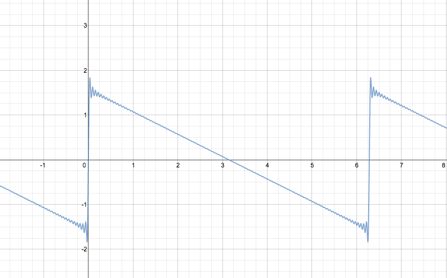
Coda: The real and imaginary parts of $\sum \frac{z^n}{n^2}$ and $\sum \frac{z^n}{n}$ also look like Fourier series, no? Here, for instance, are the graphs of $\sum_{n=1}^{100}\frac{\cos nx}{n}$ (left) and $\sum_{n=1}^{100}\frac{\sin nx}{n}$ (right):

In particular, it looks like $\sum \frac{z^n}{n}$ diverges only when $z = 1$ (where it becomes the harmonic series). Can you find the functions to which its real and imaginary parts converge away from multiples of $2\pi$? Click on the graphs and try!

an experiment…

I’ve been wanting to get LaTeX working on this blog for at least a few months now. When I first tried it, I had the impression that it would be all sorts of convoluted. Fortunately, I just found another blog post with a variety of links on how to make it simple, so I’m going to try some of them out. (See the final remark at the bottom, plus the comments, for some observations on how well this works.)

Here is what prompted my initial crise de foi regarding the marriage of LaTeX and Blogger. This past spring, I taught an “advanced calculus” course, which amounted to an introduction to (embedded) manifolds. I was a TA for this class, twice, as a graduate student, and it has some of my favorite calculus material—the kind that makes you realize what a breathtaking endeavor it is. One of the first big revelations is the nature of the derivative. I love this part of the class, and I wanted to share it.

When we first teach the derivative, we teach it as a number. We have to. It’s hard to imagine conveying anything more abstract about it when the definition already involves tangents, limits, possibly infinitesimals, and we just want to instill some level of understanding. But the purpose of the derivative—indeed, the philosophy behind all of differential calculus—is to take a curvy object and make it straight. Since we apply it to functions, the result should be a straightened function, i.e., a linear function. A linear function from $\mathbb{R}^m$ to $\mathbb{R}^n$ may be encoded by an $n \times m$ matrix. That's often convenient, but not always. Here’s a simple example that shows that sometimes it’s best to avoid matrices.

First, the matrix-free definition of the derivative. Let $U \subseteq \mathbb{R}^m$ be an open set, and let $f : U \to \mathbb{R}^n$ be a function. Then $f$ is differentiable at $\mathbf{x} \in U$ if there exists a linear function $L : \mathbb{R}^m \to \mathbb{R}^n$ such that \[ \lim_{|\mathbf{h}|\to0} \frac{|f(\mathbf{x}+\mathbf{h}) - f(\mathbf{x}) - L(\mathbf{h})|}{|\mathbf{h}|} = 0. \] If such a function $L$ exists, then it is unique, and we write $Df(\mathbf{x}) = L$.

Now consider the set of $n \times n$ matrices, and identify this set with $\mathbb{R}^{n^2}$. Define $S : \mathbb{R}^{n^2} \to \mathbb{R}^{n^2}$ by $S(A) = A^2$. If we were to write this function out in coordinates, we would see that all of the entries are polynomials, and so it is differentiable. What is its derivative at a point $A$? Note that the derivative must be a linear map from $\mathbb{R}^{n^2}$ to itself, so writing out a matrix would be fairly taxing.

Instead, we can get an idea of what the derivative should be by adding a variable matrix $H$ (presumed to be small) to the matrix $A$ and seeing the result of the function: $S(A+H) = (A+H)^2 = A^2 + AH + HA + H^2$. The part of this expression that “looks linear in $H$” is the middle two terms. Indeed, if we set $L(H) = AH + HA$, then we find \[ \lim_{|H|\to0} \frac{|(A+H)^2 - A^2 - (AH + HA)|}{|H|} = \lim_{|H|\to0} \frac{|H|^2}{|H|} = 0. \] Ah-ha! The derivative of the squaring function $S$ at $A$ is $DS(A) : H \mapsto AH + HA$! I still find this computation incredibly insightful.

What happens when $n = 1$? Then our matrix $A$ is $1 \times 1$, so it’s just a number, say $a$. The squaring map is $S(a) = a^2$, and the derivative of this map sends $h$ to $ah + ha = ah + ah = 2ah$. In the one-variable setting, we find $S'(a) = 2a$, and so this perspective on the derivative in terms of linear maps has reaffirmed the geometric meaning of the ordinary derivative: it describes the amount by which the range variable changes, infinitesimally, when the domain variable is altered infinitesimally.

Remarks:

• I learned this way of thinking about derivatives from John Hubbard through his textbook Vector Calculus, Linear Algebra, and Differential Forms: A Unified Approach. He was the instructor the first time I was a TA for this class.
• This experiment with including LaTeX seems to have been a success, provided I include the MathJax code in the post itself. Other methods which rely on altering the template have not worked for me.