big mistake or little mistake?

One of my friends shared this picture on Facebook—

(which came via mathtricks.org)—and suggested that the teacher who graded this assignment should not be teaching math at all. I suspected that the grading had fallen prey to a heavy teaching load for an elementary school teacher who might not be as comfortable as they’d like to be with mathematical concepts, so I wrote this response (which I’ve edited slightly):

The teacher is doing something rather sophisticated—solving a more general problem—which is what makes it easy to trip up on the apparent simplicity of this question. Consider the following similar questions:

“It took Marie 10 minutes to paint two boards. If she works just as fast, how long will it take her to paint three boards of the same size?”

“It took Marie 20 minutes to saw a board into 5 pieces. If she works just as fast, how long will it take her to saw another board into 6 pieces?”

In the case of the first alternative question I’ve proposed, the teacher’s reasoning would be entirely correct: 10 minutes for 2 boards means 15 minutes for three boards. Although this is not the question that’s being asked, sometimes it’s helpful to think of situations where an incorrect sequence of reasoning becomes correct in order to identify where the mistakes are.

In the case of the second alternative question I’ve proposed, think about how you would solve it. Would you divide the 20 minutes into 5 equal periods of time, or 4? Would you blame someone for dividing by 5 the first time they attempted to solve the problem? Once you figure out that what's important is the 4 cuts it takes, rather than the 5 pieces that are produced, then you can solve any such problem. For example, “If Marie takes an hour to cut a board into 6 pieces, then how long will it take to saw another board into 12 pieces?” (The answer, btw, is not 2 hours.)

The reasoning the teacher wrote on the paper is clearly of this latter kind. Their mistake is not in computation, but in choosing what aspect of the problem deserves attention, namely the cuts in the wood and not the resulting pieces. This leads to nothing more than an “off by 1” error, which is easily corrected. I would be happy to see this reasoning written on a student’s paper, because I would know that only a small correction is needed, after which the student could solve the much more general problem, thanks to a demonstrated understanding of proportion.

Math teachers have to be prepared to look for this kind of demonstrated understanding in order to hone in on where a student is making mistakes in their reasoning. This particular case is an example of someone who is teaching math, but probably also a lot of other subjects, and may or may not have training in mathematical thinking. So the more sophisticated concept—proportionality—steps in and overrides a simpler formulation of the problem, which just involves counting. This kind of mix-up is common not just in students, but among all people. Which is why I don't think it’s incompetence, but a symptom of the need for more mathematical training for teachers.

I’m curious how other math teachers would have responded to this discussion. There are certainly those in the math community that can give clearer expression to what I was trying to say. Other commenters on Facebook seemed baffled that a teacher could make this mistake in grading, but I think it’s not such a serious error in reasoning (except that the teacher should have been correcting this on students’ papers, rather than making the mistake on their own).

So, what do you think?

a bit of ex-spline-ation

Splines are piecewise-polynomial functions that interpolate between a finite set of specified points $(x_1,y_1)$, …, $(x_n,y_n)$. Cubic splines assume that each piece has at most third degree; this allows the formation of curves that appear quite smooth to the eye, as one has sufficient freedom to match both first and second derivatives at the joining points. Either the first or second derivative may be chosen freely at the first and last points; in the case of natural cubic splines, the assumption is that the second derivative vanishes at those points. I spent part of this week trying to understand how they work, and so I decided to make Desmos graphs that would illustrate how to interpolate by cubic splines for sets of three and four points.

Click on the left image to go to the graph with three points,
or the right image to go to the graph with four points.

The process I followed for three points was straightforward, if not lovely. Suppose the interpolating functions are $f_1$ and $f_2$. The assumption that $(x_1,y_1)$ and $(x_3,y_3)$ are inflection points means that $f_1$ and $f_2$ have the form \[ f_1(x) = a_1 (x - x_1)^3 + b_1 (x - x_1) + y_1 \] and \[ f_2(x) = a_2 (x - x_3)^3 + b_2 (x - x_3) + y_3 \] (think in terms of Taylor polynomials around $x_1$ and $x_3$). We need to find the coefficients $a_1, b_1, a_2, b_2$. Two conditions arise from the fact that $f_1(x_2) = f_2(x_2) = y_2$. The condition that the second derivatives match at $x_2$ implies $a_1 (x_2 - x_1) = a_2 (x_2 - x_3)$. The fourth and final condition is that the first derivatives match at $x_2$, and now the system can be solved to find $f_1$ and $f_2$ entirely.

While preparing to make a graph for four points, I came across a post on the Calculus VII blog that breaks down the whole process of computing splines in a clever and beautiful way, which also reduces the complexity of the computation. In addition, the post provides, in rough outline, a motivation for why natural cubic splines are a good choice for interpolation, and I recommend reading the whole thing. I did have to work out several of the details for myself, however, particularly since that post only deals with $x$-values spaced one unit apart. I thought that it might be useful for others to see the process that led to the formulas I use on the graph. Lots of algebra ahead.

We start with four points, $(x_1,y_1)$, $(x_2,y_2)$, $(x_3,y_3)$, and $(x_4,y_4)$, with $x_1 < x_2 < x_3 < x_4$. The first observation is that the easiest kind of interpolation is piecewise-linear, so we compute the three slopes \[ m_1 = \frac{y_2 - y_1}{x_2 - x_1}, \qquad m_2 = \frac{y_3 - y_2}{x_3 - x_2}, \qquad m_3 = \frac{y_4 - y_3}{x_4 - x_3} \] for the three segments between successive pairs of points, and the linear functions $L_1$, $L_2$, and $L_3$ corresponding to this interpolation, $L_i(x) = m_i (x - x_i) + y_i$.

Linear interpolation

The next big idea is that we want to adjust the piecewise-linear approximation by adding cubic “correction” terms $C_1$, $C_2$, and $C_3$, so that our final interpolating functions become $f_i = L_i + C_i$, $i = 1,2,3$, where $C_i(x_i) = C_i(x_{i+1}) = 0$. These latter conditions imply that $C_i$ can be written in the form \[ C_i(x) = a_i (x - x_i) (x - x_{i+1})^2 + b_i (x - x_i)^2 (x - x_{i+1}), \] which means that the first and second derivatives are \[ C_i'(x) = a_i (x - x_{i+1})^2 + 2(a_i + b_i) (x - x_i) (x - x_{i+1}) + b_i (x - x_i)^2 \] and \[ C_i''(x) = (4a_i + 2b_i) (x - x_{i+1}) + (2a_i + 4b_i) (x - x_i). \] Note also that $f_i' = m_i + C_i'$ and $f_i'' = C_i''$.

What other properties do we want these cubic functions to have?

• For the derivatives of the $f_i$s to match at $x_2$ and $x_3$, we must have $m_i + C_i'(x_{i+1}) = m_{i+1} + C_{i+1}'(x_{i+1})$ for $i = 1,2$.
• We want the second derivatives of the $C_i$s to match at $x_2$ and $x_3$ (this is the same as matching the second derivatives of the $f_i$s).
• We also require that the second derivatives be zero at the outer endpoints.

Now a curious twofold effect comes into play:

• The coefficients $a_i$ and $b_i$ are linear combinations of $z_i = C_i''(x_i)$ and $z_{i+1} = C_i''(x_{i+1})$. To wit, solving the system \[ \begin{cases} z_i &= (4 a_i + 2b_i) (x_i - x_{i+1}) \\ z_{i+1} &= (2a_i + 4 b_i) (x_{i+1} - x_i) \end{cases} \] for $a_i$ and $b_i$ yields \[ a_i = \frac{2z_i + z_{i+1}}{6 (x_i - x_{i+1})}, \qquad b_i = \frac{2z_{i+1} + z_i}{6 (x_{i+1} - x_i)} \]
• The condition that the second derivatives be equal is exceedingly simple; we have already used it implicitly in labeling them as $z_1$, $z_2$, $z_3$, $z_4$.

Our assumption at the endpoints is that $z_1 = z_4 = 0$. Thus, the whole problem reduces to finding what should be the second derivatives at the “interior” points $x_2$ and $x_3$.

Cubic correction terms

The idea of parametrizing by the second derivatives, after removing the “linear” effects, is where the beauty and cleverness in this solution lie. We use the assumption about matching first derivatives (a linear condition in the coefficients) to set up the remaining conditions on the second derivatives (which themselves depend linearly on the coefficients). Looking back, this is essentially what I did for three points, but I missed out on dealing with the linear effects separately, so I had to solve for three variables simultaneously. At this point, we only need to solve for two: $z_2$ and $z_3$.

Since $C_i'(x_i) = a_i (x_i - x_{i+1})^2 = \frac{1}{6} (2z_i + z_{i+1})(x_i - x_{i+1})$ and $C_i'(x_{i+1}) = b_i (x_{i+1} - x_i)^2 = \frac{1}{6} (2z_{i+1} + z_i)(x_{i+1} - x_i)$, the equations $m_i + C_i'(x_{i+1}) = m_{i+1} + C_{i+1}'(x_{i+1})$ become \[ \begin{cases} (x_2 - x_1) (2z_2 + z_1) + (x_3 - x_2) (2 z_2 + z_3) = 6(m_2 - m_1) \\ (x_3 - x_2) (2z_3 + z_2) + (x_4 - x_3) (2 z_3 + z_4) = 6(m_3 - m_2) \end{cases} \] (in this form, it is easy to see how to generalize to $n$ points, and it shows the origin of what the other post called the “tridiagonal” form of the system). Now we set $z_1$ and $z_4$ to zero and solve for $z_2$ and $z_3$. For this two-variable system it isn’t too bad to write down the explicit solution, which is what is used in the Desmos graph: \begin{gather*} z_2 = 6 \frac{3 m_2 x_2 + 2 m_1 x_4 + m_3 x_2 - 2 m_1 x_2 - 2 m_2 x_4 - m_2 x_3 - m_3 x_2}{(x_2 + x_3)^2 - 4 (x_1 x_2 + x_3 x_4 - x_1 x_4)} \\ z_3 = 6 \frac{3 m_2 x_3 + 2 m_3 x_1 + m_1 x_2 - 2 m_2 x_1 - 2 m_3 x_3 - m_1 x_3 - m_2 x_2}{(x_2 + x_3)^2 - 4 (x_1 x_2 + x_3 x_4 - x_1 x_4)} \end{gather*}

In this graph, blue plus green equals red.

Finally, to check that we have actually created a spline with the desired properties, we can look at the graphs of the first and second derivatives to make sure they’re continuous.

The spline is red. The first derivative is purple, and the second derivative is orange.

Notice that the second derivative is piecewise linear (naturally, since the spline is piecewise cubic) and zero at the endpoints (as we chose it to be). I particularly like seeing how the derivatives change as the points are moved.

Anyway, I learned a lot from putting together the graphs, and almost as much from writing this post. I think there are lots of interesting explorations one could do with these graphs, but for now I’ll just release them to the wild and hope people enjoy them!

P.S. Please pardon the bad pun in the title. I’m working on making my post titles more… interesting?

be careful with computers

This week in my calculus class, we were studying examples of separable differential equations: exponential growth and decay, Newton’s Law of Heating and Cooling, and the logistic model, respectively \[ \frac{dy}{dt} = ky, \qquad \frac{dy}{dt} = k(M-y), \qquad\text{and}\qquad \frac{dy}{dt} = ky\left(1-\frac{y}{L}\right). \]

We explored how the shapes of solutions depend on the parameters in the equations, which parameters are most physically meaningful in various situations, and what extra parameters appear in the course of solving them.

I had several goals for this course of study:

• to show the versatility of differential equations in modeling physical situations;
• to show the usefulness of integration techniques for solving real-world problems;
• to practice understanding the behavior of solutions to differential equations by examining the equations themselves;
• to get students more familiar with Wolfram Alpha and Desmos as computational tools.

This last goal led to a curious discovery, which is what prompted me to write this post.

In the age of widely-accessible computer algebra systems, we are finally freed from spending a month in calculus class mastering techniques of integration. Substitution and integration by parts are indispensable, but as far as I’m concerned, the rest of the methods are used infrequently enough that students should be made aware that other techniques exist and they can learn them when needed. In particular, solving the logistic equation is about the only reason I can conjure to justify learning partial fractions in introductory calculus. So we learned how to compute partial fractions for a rational function with two linear factors in the denominator. Here’s how it gets used.

First, rearrange the logistic equation a bit and separate variables to get \[ \frac{dy}{y(y-L)} = -\frac{k}{L}dt. \] The right side clearly integrates to $-\frac{k}{L}t$. Using partial fractions, the integral of the left side is \[ \int\frac{dy}{y(y-L)} = \int \frac{1}{L} \frac{dy}{y - L} - \int\frac{1}{L} \frac{dy}{y} = \frac{1}{L} \big( \ln|y - L| - \ln|y| \big) = \frac{1}{L} \ln \left|\frac{y - L}{y}\right|. \] Tossing in the ever-present arbitrary constant of integration $+C$ (which really matters very little until one starts solving differential equations, as here), we have \[ \frac{1}{L} \ln \left|\frac{y - L}{y}\right| = -\frac{k}{L}t + C. \] Multiply both sides by $L$ and exponentiate both sides to get \[ \left|\frac{y - L}{y}\right| = e^{-kt + LC} = e^{LC} e^{-kt}. \] Now, $e^{LC}$ is always positive, but when we drop the absolute value signs, we get \[ \frac{y - L}{y} = Be^{-kt}, \] where $B$ can be either positive or negative. Finally, solve for $y$: \[ y = \frac{L}{1 + Ae^{-kt}} \] (where $A = -B$). Technically, throughout this process we had to assume that $y \ne 0$ and $y \ne L$. That’s okay, though, because $y = 0$ and $y = L$ are evident as equilibrium (constant) solutions from the equation itself.

There are three qualitatively different behaviors that solutions to the logistic equation can have, depending on their initial values.

1. The solutions $y = 0$ and $y = L$, as mentioned above, are constant.
2. A solution that starts out between $0$ and $L$ will increase over time, approaching the value $L$ asymptotically. This behavior corresponds to $A > 0$ in the solution above.
3. A solution that starts out above $L$ will decrease over time, again approaching the value $L$ asymptotically. This behavior corresponds to $A < 0$ in the solution above.

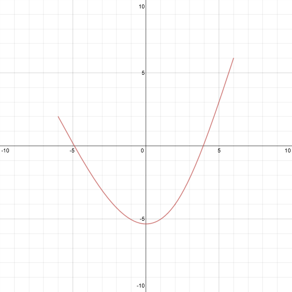
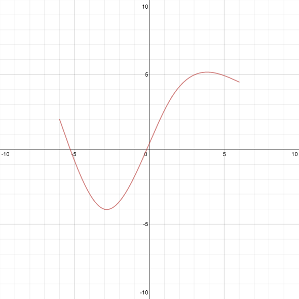
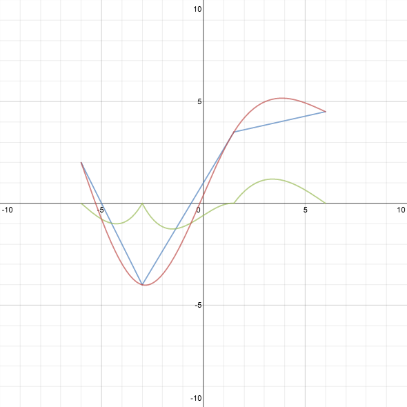
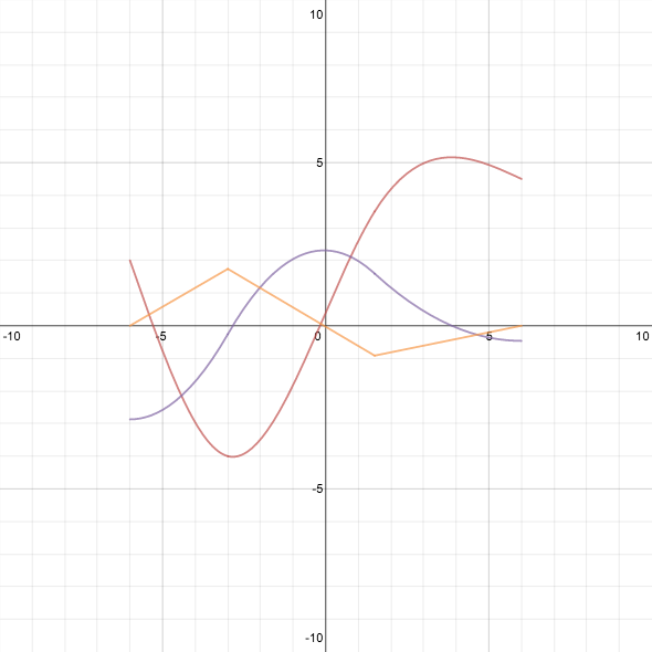
The case of an initial value below zero is generally not physically meaningful, and in any case it follows the same formula as 3. (See the red curve in the third image at the top.) The most interesting solutions are type 2, whose graphs follow what Wikipedia describes as a “sigmoid” shape (the blue curve in the image at top). These are the solutions that provide the most meaningful applications of the logistic equation: growth in a constrained environment.

So far, so good, and I haven’t said anything that isn’t easily found elsewhere. But before we solved the logistic equation by hand, I wanted my students to explore the solutions graphically, so I had them plug the equation into Wolfram Alpha. Here’s the solution it provides: \[ y(t) = \frac{L e^{c_1 L+k t}}{e^{c_1 L+k t}-1}. \] However, if you plot this solution (link goes to a Desmos graph) and vary the parameters (particularly $c_1$, since $k$ and $L$ are constants given in the equation), you will only see one kind of solution: the third kind. Type 2 solutions, the most interesting ones, don’t even show up in Wolfram Alpha’s formula! What’s going on?

If you sign in to Wolfram Alpha, you can have it produce step-by-step solutions. The results from this query:

This doesn’t look so different from our solution: separate variables, integrate, solve for $y$. In W|A, $\log$ denotes the natural logarithm, so nothing’s amiss there. What’s changed?

It’s a small thing, one that could easily be missed, even if you’re looking step-by-step. A hint comes from the placement of the additional parameter that arises from the constant of integration: in our solution, this parameter ended up in front of the exponential function, whereas Wolfram Alpha left it in the exponent. That’s not really the issue though… ah, there it is:

After integrating, there’s no absolute value inside the logarithm (gasp!). I know, we try to convince our students time and time again that the standard antiderivative of $\frac{1}{x}$ is $\ln|x|$, and here Wolfram is leaving out the absolute value. And it turns out to make a difference—go back and read the solution we went through, and you’ll see that the moment the absolute value was dropped from the equation is precisely when our formula gained the flexibility to accommodate both type 2 and type 3 solutions. Wolfram Alpha missed solutions by leaving out the absolute value.

This isn’t all that disastrous. I know that Wolfram Alpha generally assumes complex arithmetic, in which case the logarithm requires a branch cut anyway. It also assumes a fair amount of mathematical sophistication on the part of its users. It wasn’t too hard for me to figure out why we didn’t get the answer we expected. [For more on these points, see the addendum, below.] But this example does suggest caution when we try to use W|A for educational purposes. In fact, it reinforces the message that as we’re training our students to use computing tools, we need to make sure they’re doing so intelligently. One doesn’t need to fully anticipate the answer provided, but one should have some idea of what to expect, to check the answer’s reasonableness.

I’m also not arguing that one has to be a stickler about constants of integration or absolute values in logarithms from the moment that they are introduced. Such matters are generally secondary in the early days of learning integration. But when motivation for such secondary matters naturally arises in examples of interest, that should be seized.

Addendum (2/16): When I first posted this, I suggested that it was evidence of a bug in Wolfram Alpha. Later I realized that this is not technically the case, because with complex numbers, Euler’s formula shows that we can get all of the solutions; for instance, if we let $c_1 = i\pi + c_2$, then Wolfram Alpha’s answer becomes $L e^{c_2+k t}/(e^{c_2+k t}+1)$. Indeed, if we add the initial condition $y(0) = L/2$, then W|A returns $y(t) = Le^{kt}/(e^{kt}+1)$, as expected. It’s not enough, however, to specify that the equation be solved over the reals; doing so gives the same answer as at first. The pedagogical points I made about using technology still stand. They are perhaps even made stronger, as defaulting to computations over the complex numbers often produces results that can be confusing for students. This doesn’t mean we should avoid using such tools, but we should prepare our students to adapt to unexpected output.