Splines are piecewise-polynomial functions that interpolate between a finite set of specified points $(x_1,y_1)$, …, $(x_n,y_n)$. Cubic splines assume that each piece has at most third degree; this allows the formation of curves that appear quite smooth to the eye, as one has sufficient freedom to match both first and second derivatives at the joining points. Either the first or second derivative may be chosen freely at the first and last points; in the case of natural cubic splines, the assumption is that the second derivative vanishes at those points. I spent part of this week trying to understand how they work, and so I decided to make Desmos graphs that would illustrate how to interpolate by cubic splines for sets of three and four points.
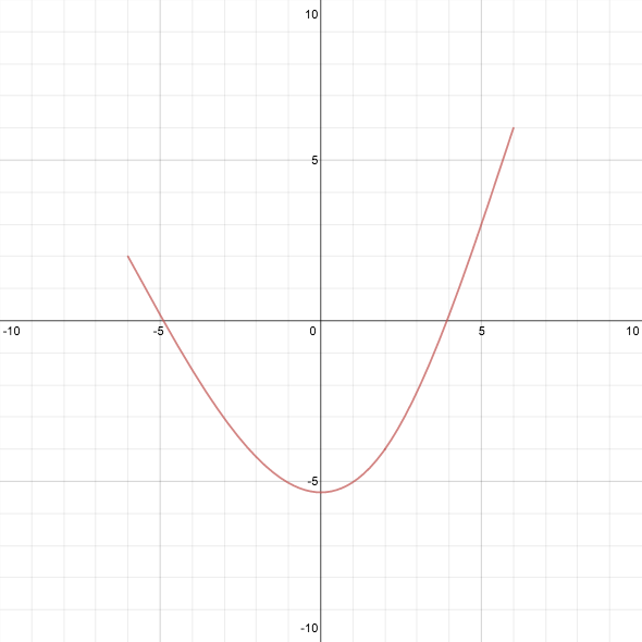
Click on the left image to go to the graph with three points,
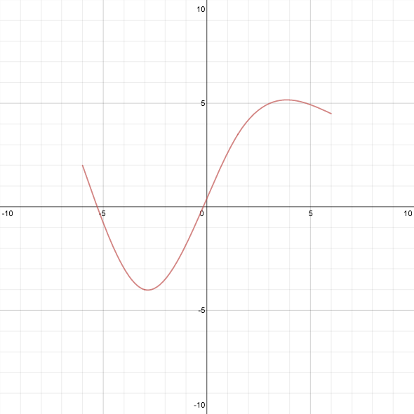
or the right image to go to the graph with four points.
The process I followed for three points was straightforward, if not lovely. Suppose the interpolating functions are $f_1$ and $f_2$. The assumption that $(x_1,y_1)$ and $(x_3,y_3)$ are inflection points means that $f_1$ and $f_2$ have the form \[ f_1(x) = a_1 (x - x_1)^3 + b_1 (x - x_1) + y_1 \] and \[ f_2(x) = a_2 (x - x_3)^3 + b_2 (x - x_3) + y_3 \] (think in terms of Taylor polynomials around $x_1$ and $x_3$). We need to find the coefficients $a_1, b_1, a_2, b_2$. Two conditions arise from the fact that $f_1(x_2) = f_2(x_2) = y_2$. The condition that the second derivatives match at $x_2$ implies $a_1 (x_2 - x_1) = a_2 (x_2 - x_3)$. The fourth and final condition is that the first derivatives match at $x_2$, and now the system can be solved to find $f_1$ and $f_2$ entirely.
While preparing to make a graph for four points, I came across a post on the Calculus VII blog that breaks down the whole process of computing splines in a clever and beautiful way, which also reduces the complexity of the computation. In addition, the post provides, in rough outline, a motivation for why natural cubic splines are a good choice for interpolation, and I recommend reading the whole thing. I did have to work out several of the details for myself, however, particularly since that post only deals with $x$-values spaced one unit apart. I thought that it might be useful for others to see the process that led to the formulas I use on the graph. Lots of algebra ahead.
We start with four points, $(x_1,y_1)$, $(x_2,y_2)$, $(x_3,y_3)$, and $(x_4,y_4)$, with $x_1 < x_2 < x_3 < x_4$. The first observation is that the easiest kind of interpolation is piecewise-linear, so we compute the three slopes \[ m_1 = \frac{y_2 - y_1}{x_2 - x_1}, \qquad m_2 = \frac{y_3 - y_2}{x_3 - x_2}, \qquad m_3 = \frac{y_4 - y_3}{x_4 - x_3} \] for the three segments between successive pairs of points, and the linear functions $L_1$, $L_2$, and $L_3$ corresponding to this interpolation, $L_i(x) = m_i (x - x_i) + y_i$.
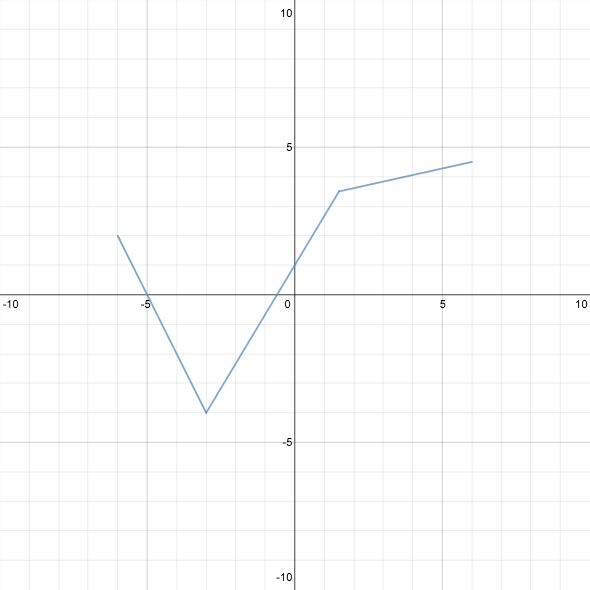
Linear interpolation
The next big idea is that we want to adjust the piecewise-linear approximation by adding cubic “correction” terms $C_1$, $C_2$, and $C_3$, so that our final interpolating functions become $f_i = L_i + C_i$, $i = 1,2,3$, where $C_i(x_i) = C_i(x_{i+1}) = 0$. These latter conditions imply that $C_i$ can be written in the form \[ C_i(x) = a_i (x - x_i) (x - x_{i+1})^2 + b_i (x - x_i)^2 (x - x_{i+1}), \] which means that the first and second derivatives are \[ C_i'(x) = a_i (x - x_{i+1})^2 + 2(a_i + b_i) (x - x_i) (x - x_{i+1}) + b_i (x - x_i)^2 \] and \[ C_i''(x) = (4a_i + 2b_i) (x - x_{i+1}) + (2a_i + 4b_i) (x - x_i). \] Note also that $f_i' = m_i + C_i'$ and $f_i'' = C_i''$.
What other properties do we want these cubic functions to have?
- For the derivatives of the $f_i$s to match at $x_2$ and $x_3$, we must have $m_i + C_i'(x_{i+1}) = m_{i+1} + C_{i+1}'(x_{i+1})$ for $i = 1,2$.
- We want the second derivatives of the $C_i$s to match at $x_2$ and $x_3$ (this is the same as matching the second derivatives of the $f_i$s).
- We also require that the second derivatives be zero at the outer endpoints.
- The coefficients $a_i$ and $b_i$ are linear combinations of $z_i = C_i''(x_i)$ and $z_{i+1} = C_i''(x_{i+1})$. To wit, solving the system \[ \begin{cases} z_i &= (4 a_i + 2b_i) (x_i - x_{i+1}) \\ z_{i+1} &= (2a_i + 4 b_i) (x_{i+1} - x_i) \end{cases} \] for $a_i$ and $b_i$ yields \[ a_i = \frac{2z_i + z_{i+1}}{6 (x_i - x_{i+1})}, \qquad b_i = \frac{2z_{i+1} + z_i}{6 (x_{i+1} - x_i)} \]
- The condition that the second derivatives be equal is exceedingly simple; we have already used it implicitly in labeling them as $z_1$, $z_2$, $z_3$, $z_4$.
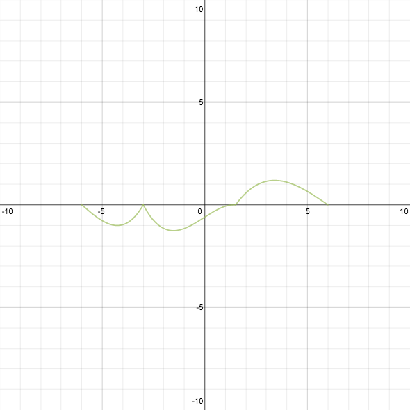
Cubic correction terms
The idea of parametrizing by the second derivatives, after removing the “linear” effects, is where the beauty and cleverness in this solution lie. We use the assumption about matching first derivatives (a linear condition in the coefficients) to set up the remaining conditions on the second derivatives (which themselves depend linearly on the coefficients). Looking back, this is essentially what I did for three points, but I missed out on dealing with the linear effects separately, so I had to solve for three variables simultaneously. At this point, we only need to solve for two: $z_2$ and $z_3$.
Since $C_i'(x_i) = a_i (x_i - x_{i+1})^2 = \frac{1}{6} (2z_i + z_{i+1})(x_i - x_{i+1})$ and $C_i'(x_{i+1}) = b_i (x_{i+1} - x_i)^2 = \frac{1}{6} (2z_{i+1} + z_i)(x_{i+1} - x_i)$, the equations $m_i + C_i'(x_{i+1}) = m_{i+1} + C_{i+1}'(x_{i+1})$ become \[ \begin{cases} (x_2 - x_1) (2z_2 + z_1) + (x_3 - x_2) (2 z_2 + z_3) = 6(m_2 - m_1) \\ (x_3 - x_2) (2z_3 + z_2) + (x_4 - x_3) (2 z_3 + z_4) = 6(m_3 - m_2) \end{cases} \] (in this form, it is easy to see how to generalize to $n$ points, and it shows the origin of what the other post called the “tridiagonal” form of the system). Now we set $z_1$ and $z_4$ to zero and solve for $z_2$ and $z_3$. For this two-variable system it isn’t too bad to write down the explicit solution, which is what is used in the Desmos graph: \begin{gather*} z_2 = 6 \frac{3 m_2 x_2 + 2 m_1 x_4 + m_3 x_2 - 2 m_1 x_2 - 2 m_2 x_4 - m_2 x_3 - m_3 x_2}{(x_2 + x_3)^2 - 4 (x_1 x_2 + x_3 x_4 - x_1 x_4)} \\ z_3 = 6 \frac{3 m_2 x_3 + 2 m_3 x_1 + m_1 x_2 - 2 m_2 x_1 - 2 m_3 x_3 - m_1 x_3 - m_2 x_2}{(x_2 + x_3)^2 - 4 (x_1 x_2 + x_3 x_4 - x_1 x_4)} \end{gather*}
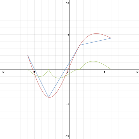
In this graph, blue plus green equals red.
Finally, to check that we have actually created a spline with the desired properties, we can look at the graphs of the first and second derivatives to make sure they’re continuous.
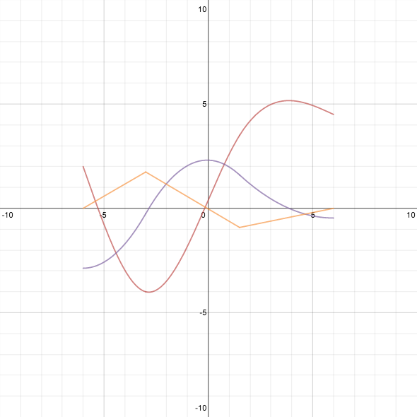
The spline is red. The first derivative is purple, and the second derivative is orange.
Notice that the second derivative is piecewise linear (naturally, since the spline is piecewise cubic) and zero at the endpoints (as we chose it to be). I particularly like seeing how the derivatives change as the points are moved.
Anyway, I learned a lot from putting together the graphs, and almost as much from writing this post. I think there are lots of interesting explorations one could do with these graphs, but for now I’ll just release them to the wild and hope people enjoy them!
P.S. Please pardon the bad pun in the title. I’m working on making my post titles more… interesting?
1 comment:
This is a gold mine, I have been studying it for several days trying to write code behind an algorithm I have been working on. Is this post still active? I am stuck and would like to ask for your assistance. I cant find anything else on the web that comes as close as this....
Post a Comment